Cleaning and Conversion of Raw or Improper Data into Proper Data

   INTRODUCTION 

 The purpose of using excel is to analyze data and make informed decision. The analysis is based on the underlying data and its proper formatting and it becomes even more important as the input data gets larger. If you are doing the analysis, it is likely that some one else is doing the data entry for you or you are importing data from other sources such as *.csv or *.txt format over which you have no control. In both the cases, there are chances that the raw data that you will get is not perfectly suitable of analysis right away. In most cases, there are some inadvertent error which are made during data entry which require some sanitation or cleaning before the analysis. 

You may face common errors as under:

• Inclusion of non-printable characters such as line break. This causes the text data to appear in zig zag manner and it is frustrating to remove such characters manually. 
• Multiple spaces or extra spaces in a sentence which can make your life difficult as the word "ABC", " ABC" and "ABC " are all treated differently by excel. It is not easy to detect such extra spaces especially if they are on the end. Again, needless to say, removing spaces manually is highly annoying.
• Numbers entered as text. One of the most common mistake I have seen people committing. Sometimes people want to write Rs 100/- or 50 Kg or 25 Km/hr but instead of using the proper number format they end up entering it as a text. In some cases, an apostrophe is added which also converts number as text.
  
• Sometimes when you import data from other sources, multiple blank rows or columns get inserted in between the input data and if the data source is large it is untenable to delete blank rows/columns manually.

 Solution for Non printable and Extra Spaces

To remove the non-printable characters, excel has a function known as 'CLEAN' function which takes the text input and removes all the non-printable characters (first 32 ASCII characters). The example is as under:

 

 In the above example, there are line breaks when data was copied from other sources (in this case from PDF) and as you can see in the formula bar, the line breaks are neither required nor are they at proper places. Using Clean function help removes such characters. 

Another excel function, TRIM, is used to remove the extra spaces from a sentence. Many a times there are multiple spaces and the TRIM function gets rid of them efficiently.

Here, you can see extra spaces in the column C along with the length of string. The TRIM function [TRIM(C3)] removes the extra spaces and converts into a nice word with single spaces. Compare the length of string before and after using TRIM. 

In most practical cases,when you get the improper data set, it is advisable to use the combination of CLEAN and TRIM function to get the good results. A combination example is given below:

As you can see, the non printable character and the extra spaces are removed in a one go and the data in column D is much presentable than what is in column C. 

 Solution for Numbers entered as Text

The Excel, by default, aligns the number entered to the right and in case of Text the default alignment is to the left and the Logical Values are centrally aligned. The image below shows this:

 An easy visual check to see if the number is entered as text is to check the alignment provided that the alignment was not formatted manually. 

First of all check the data category type and it should be set as Number or General. To convert a text which is entered as number, you may use the excel function NUMBERVALUE (it is available for excel version 2013 and later). 

Another way to convert number entered as text to number is by using math operation. You can add 0 to the text or multiply by one as it will not change the underlying value but convert the text to the number with right alignment. This will work in all versions of excel. The following example demonstrates both approaches:

If you have entered number along with units, the excel will treat that as a text. For instance, if you are entering the weight of individuals in Kg and you are entering data 50 Kg, 65 Kg etc then you can't do any calculation on it. The better way to show the units is to use the custom number formatting which changes the appearance of the number without making any underlying change. In other words, the number entered as a number and the custom formatting takes care of adding units (prefix or suffix) as you want. 

Steps to follow:

    1. Select the range where you want to add numbers with units :

 

    2. Press Ctrl + 1. This will open the number format dialog box and then select Custom category shown below.

   

    3.    The add the this custom number format string # "Kg" into the 'Type Text Box' as shown below.

    4.  Then click OK button and the following result may appear:

 

 You can use any units such as lb, km/hr, miles etc simply by replacing the "Kg" with other units. If you want to prefix something such as Rs then put "Rs" ahead of #. 

This not only saves your time by not manually entering the units but also allow you to do all kinds of mathematical operation or analysis you may want. Remember that the custom number formatting doesn't change the underlying value but only acts as facade for appearance.

 
Solution for removing blank rows

This happens mostly when you import data from CSV or TXT format. The excel works best with proper data sets i.e. there should not be any entirely empty row in your data set otherwise the data set will not be visible to excel in its entirety. 

Now, removing blank rows and columns manually will be quite frustrating. The most fool-proof way of doing this (without using VBA) is to use a helper column to concatenate all the columns of each row in to helper cell and then using filter to identify entirely blank rows and then deleting all in a one go. 

Illustration:

Consider the following data set:

 

The empty cell have been highlighted in yellow color. We want to delete only entirely empty rows. Hence only Row 6 and Row 9 should be deleted. For this we need to create a helper column which we have done in Column H. 

 

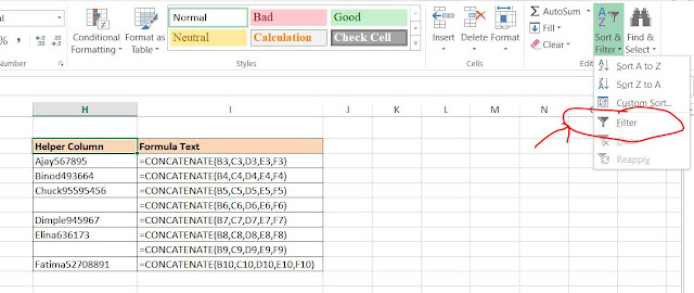
 We have used concatenate formula to combine all the columns of each row into one cell. Only the entirely empty rows will give out empty string after using CONCATENATE. Here Cell H6 and H9. Thereafter, we will apply filter to helper column. To do that select the Cell H2 with the text Helper Column and select filter under Home Tab as shown below.

 

The filter icon will appear on the cell H2. Click on it and a drop down will appear and you have to select the blank checkbox as shown below.

 Ensure that only (Blanks) check box is selected and other options are de-selected and then click OK. You will see only the blank rows of the Data Set. 

Just Delete those rows and your data set will be without any blank row which may hamper your analysis as shown below.

 

 Lastly, clear the filter from the Helper column and your data set will now look like this:

 

Now, your data set is ready for analysis.

****